Spectral Graph Matching Methods: Umeyama Algorithm

Usage

graph_match_Umeyama(A, B, seeds = NULL, similarity = NULL)

Arguments

A: A matrix, igraph object, or list of either.
B: A matrix, igraph object, or list of either.
seeds: A vector of integers or logicals, a matrix or a data frame. If the seed pairs have the same indices in both graphs then seeds can be a vector. If not, seeds must be a matrix or a data frame, with the first column being the indices of \(G_1\) and the second column being the corresponding indices of \(G_2\).
similarity: A matrix. An n-by-n matrix containing vertex similarities.

Value

graph_match_Umeyama returns an object of class "graphMatch" which is a list containing the following components:

corr_A: matching correspondence in \(G_1\)
corr_B: matching correspondence in \(G_2\)
soft: the functional similarity score matrix with which one can extract more than one matching candidates
lap_method: Choice for solving the LAP
seeds: a vector of logicals indicating if the corresponding vertex is a seed

References

S. Umeyama (1988), An eigendecomposition approach to weighted graph matching problems. IEEE TPAMI. USA, pages 695-703.

Examples

# match G_1 & G_2 using Umeyama algorithm
G <- sample_correlated_gnp_pair(10, .9, .5)
g1 <- G$graph1
g2 <- G$graph2
startm <- matrix(0, 10, 10)
diag(startm)[1:4] <- 1

GM_Umeyama <- gm(g1, g2, similarity = startm, method = "Umeyama")
GM_Umeyama
#> gm(A = g1, B = g2, similarity = startm, method = "Umeyama")
#> 
#> Match (10 x 10):
#>    corr_A corr_B
#> 1       1      1
#> 2       2      2
#> 3       3      3
#> 4       4      4
#> 5       5      5
#> 6       6      8
#> 7       7      6
#> 8       8      9
#> 9       9      7
#> 10     10     10
# generate the corresponding permutation matrix
GM_Umeyama[]
#> 10 x 10 sparse Matrix of class "dgCMatrix"
#>                          
#>  [1,] 1 . . . . . . . . .
#>  [2,] . 1 . . . . . . . .
#>  [3,] . . 1 . . . . . . .
#>  [4,] . . . 1 . . . . . .
#>  [5,] . . . . 1 . . . . .
#>  [6,] . . . . . . . 1 . .
#>  [7,] . . . . . 1 . . . .
#>  [8,] . . . . . . . . 1 .
#>  [9,] . . . . . . 1 . . .
#> [10,] . . . . . . . . . 1

summary(GM_Umeyama, g1, g2)
#> Call: gm(A = g1, B = g2, similarity = startm, method = "Umeyama")
#> 
#> # Matches: 10, # Seeds:  0, # Vertices:  10, 10
#>                         
#>   common_edges 15.000000
#>  missing_edges  9.000000
#>    extra_edges  8.000000
#>          fnorm  5.830952
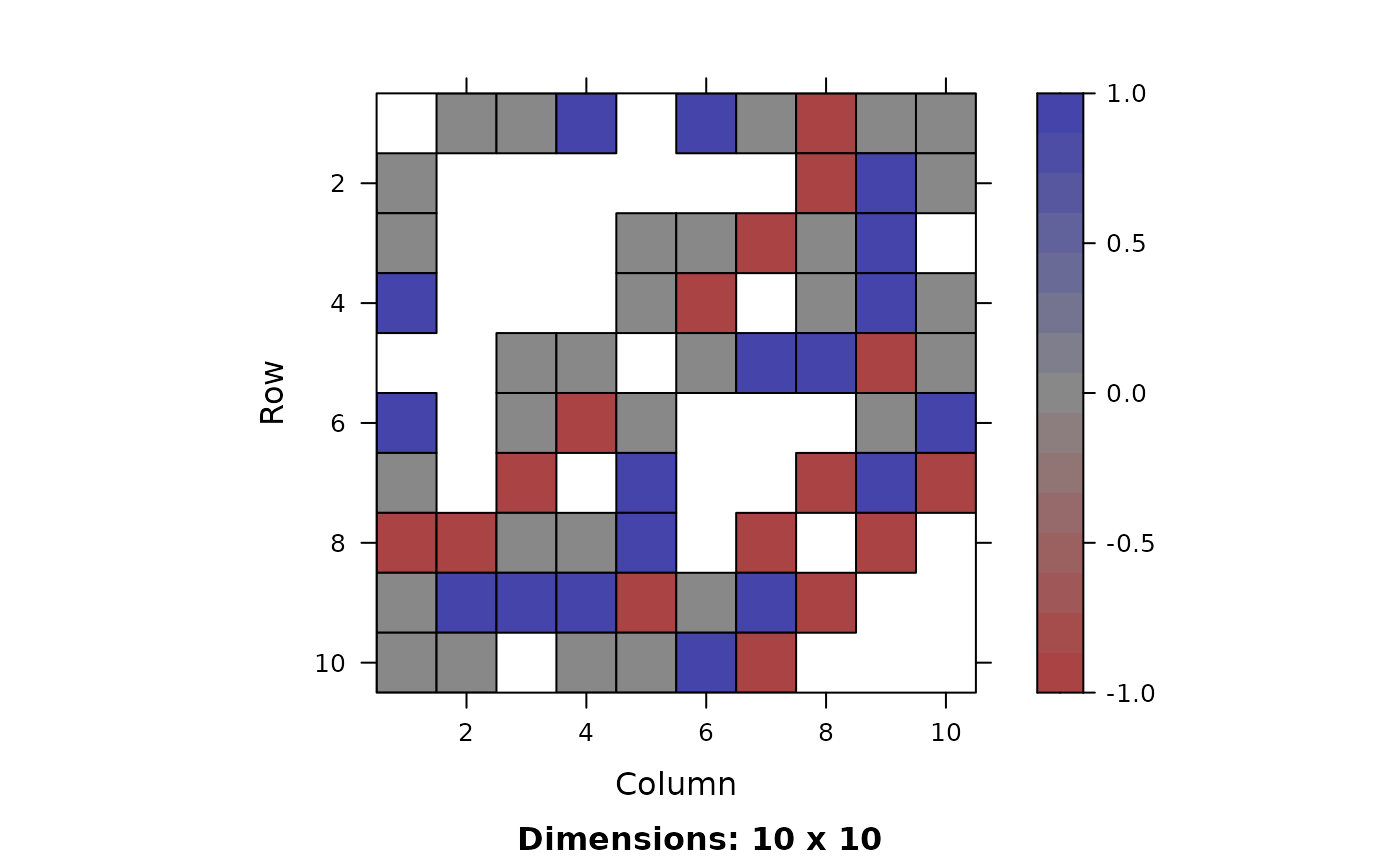
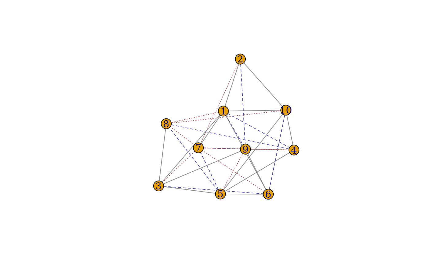
# visualize the edge-wise matching performance
plot(g1, g2, GM_Umeyama)

plot(g1[], g2[], GM_Umeyama)